Mathematical Equations

Mathematical Equations shows how to visualize mathematical equations in QML with all the available graph types. It also shows how to integrate QtQuick3D scene into a graph and how to adjust the outlook of the graph using ExtendedSceneEnvironment.

For more information about basic QML application functionality, see Simple Scatter Graph.

Running the Example

To run the example from Qt Creator, open the Welcome mode and select the example from Examples. For more information, visit Building and Running an Example.

Setting up

The data for all the graph types can be stored in a common ListModel:

ListModel {
    id: dataModel
}

The model is set for each graph type in the graph series:

Surface3DSeries {
    id: surfaceSeries
    itemLabelFormat: "(@xLabel, @zLabel): @yLabel"

    ItemModelSurfaceDataProxy {
        itemModel: dataModel
        columnRole: "xPos"
        yPosRole: "yPos"
        rowRole: "zPos"
    }
}
...
Bar3DSeries {
    id: barSeries
    itemLabelFormat: "@colLabel, @rowLabel: @valueLabel"

    ItemModelBarDataProxy {
        itemModel: dataModel
        columnRole: "xPos"
        valueRole: "yPos"
        rowRole: "zPos"
    }
}
...
Scatter3DSeries {
    id: scatterSeries
    itemLabelFormat: "(@xLabel, @zLabel): @yLabel"
    mesh: Abstract3DSeries.Mesh.Point

    ItemModelScatterDataProxy {
        itemModel: dataModel
        xPosRole: "xPos"
        yPosRole: "yPos"
        zPosRole: "zPos"
    }
}

Setting the roles allows the data in the model to be mapped to the corresponding axes automatically.

Parsing the equation

The equation can be typed into the text field using the following operators and mathematical functions, and the required characters for using those functions:

There is support for x and y as the parameters, as the data handled has two axes and the value. The equation may have spaces around the operators, so both of the following styles are fine:

• x^2+y^2
• x ^ 2 + y ^ 2

The equation is parsed using a JavaScript equation parser and calculator, which is imported to QML:

import "calculator.js" as Calc

The calculator was posted to Stack Overflow by tanguy_k in TypeScript, and has been converted to JavaScript to be usable from QML.

The equation parameters are filled in every time the equation changes or the column or row counts are updated.

Looping the rows and columns:

for (i = xValues.first.value; i <= xValues.second.value; ++i) {
    for (j = zValues.first.value; j <= zValues.second.value; ++j)
        addDataPoint(i, j)
}

Filling in the values for x and y:

function addDataPoint(i, j) {
    var filledEquation = equation.text.replace("x", i)
    filledEquation = filledEquation.replace("y", j)
    ...

The equation is then passed to the JavaScript calculator to get the result, which is then added to the data model by inserting them into the defined roles:

try {
    var result = Calc.calculate(filledEquation)
    dataModel.append({"xPos": i, "yPos": result, "zPos": j})
}

In case there is a mistake or an unknown operator or mathematical function in the equation, the error thrown by the calculator is caught, and an error dialog is shown:

MessageDialog {
    id : messageDialog
    title: qsTr("Error")
    text: qsTr("Undefined behavior")
    ...

Displaying the error message from the calculator:

catch(msg) {
    messageDialog.informativeText = msg.toString()
    messageDialog.open()
}

Graphs

The same data model is used for all three graph types. There are some differences between setting the graphs up, though.

Surface

Surface graph is used to show the data without any specific modifications. It renders the equation at each row and column with the calculation result.

The only changes done are setting the axis segment counts:

axisX.segmentCount: 10
axisZ.segmentCount: 10
axisY.segmentCount: 10

A range gradient is set for the theme to highlight the high and low values:

theme : GraphsTheme {
    id: surfaceTheme
    colorStyle: GraphsTheme.ColorStyle.RangeGradient
    baseGradients: [ gradient1 ]
    plotAreaBackgroundVisible: false
}

The gradient itself is defined elsewhere to be usable by other themes.

Bars

For bars, range gradient is also used. The gradient utilizes slight transparency to make seeing the values easier without rotating the graph that much. A slider has been added to control the level of transparency.

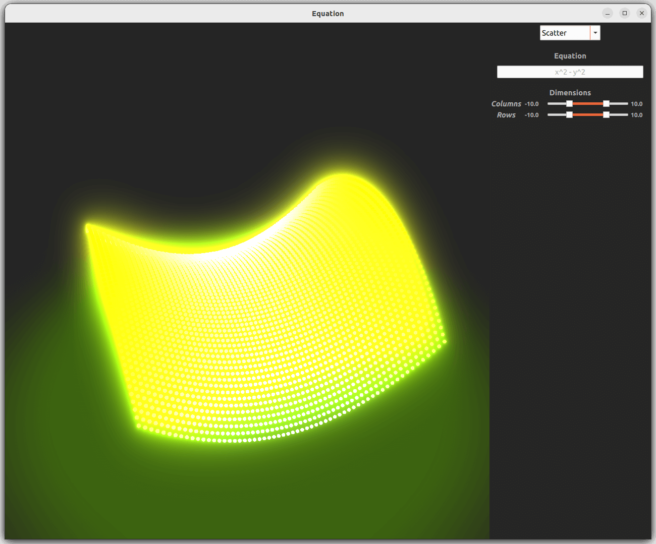
Scatter

For scatter, the theme is adjusted a bit more in preparation for the QtQuick3D integrations.

First, it will use a different gradient from the other two. Then, a dark color scheme is forced on, unlike the other two, which use system preference. Finally, plot area background, labels, and grid are hidden by setting their visibility to false.

Scatter graph is good at showing a large number of data points, which is why 3 data points are added for each "row" and "column". Scatter does not have the concept of rows and columns, which is why this can be done:

for (var i = xValues.first.value; i <= xValues.second.value; i += 0.333) {
    for (var j = zValues.first.value; j <= zValues.second.value; j += 0.333)
        addDataPoint(i, j)
}

Because the scatter graph has a lot more data points than the other two graphs, it is better to use the lightest available mesh type for the points:

mesh: Abstract3DSeries.Mesh.Point

Integrating a QtQuick3D scene

For the QtQuick3D types to be found, it has to be imported into the QML:

import QtQuick3D

A QtQuick3D scene can be imported into the graph using the importScene property. The scene can be a combination of Models, Lights, reflection probes, and other Nodes contained in a root Node. In this example, only a rectangle with an opacity map is added:

importScene: Node {
    Model {
        scale: Qt.vector3d(0.1, 0.1, 0.1)
        source: "#Rectangle"
        y: -2
        eulerRotation.x: -90
        materials: [
            PrincipledMaterial {
                baseColor: "#373F26"
                opacityMap: Texture {
                    source: "qrc:/images/opacitymap.png"
                }
            }
        ]
    }
}

Changing the outlook using QtQuick3D

For the ExtendedSceneEnvironment to be found, the following import is needed:

import QtQuick3D.Helpers

To override the default scene environment of the graph, the environment property is added with an ExtendedSceneEnvironment. In this case, backgroundMode, clearColor, and tonemapMode are set. In addition, glow is enabled. Adding post-processing effects like glow requires setting the tone map mode to TonemapModeNone.

environment: ExtendedSceneEnvironment {
    backgroundMode: ExtendedSceneEnvironment.Color
    clearColor: scatterTheme.backgroundColor
    tonemapMode: ExtendedSceneEnvironment.TonemapModeNone
    glowEnabled: true
    ...

To make the glow strong, several other related properties are set.

Example project @ code.qt.io